Использование в медицине поперечного эффекта
Доплера для ультразвуковой диагностики
сердечно-сосудистой системы

Олег Е. Акимов

Медики, занятые решением конкретных практических задач, связанных с лечением сердечно-сосудистых заболеваний, легко перешагивают через препоны, выставленные релятивистами. Последние, как известно, утверждают, будто никакого поперечного эффекта Доплера для акустических волн существовать не может. Но инженеры-медики, разрабатывающие аппаратуру для ультразвуковой диагностики сердечно-сосудистой системы, доказывают обратное. Пусть их теоретические рассуждения не всегда и во всём точны, тем не менее, они регистрируют и вполне успешно используют факт, который, казалось бы, абсолютно не возможен с точки зрения релятивистской теории. Кратко напомним суть проблемы, которая более полно изложена на следующих страницах:

• Введение в акустику. Природа звука и ультразвука
• Введение в конструктивную физику
• О формуле, описывающей классический эффект Доплера
• Ошибочность релятивистской формулы Доплера
• Квантовая теория Доплер-эффекта
• Эксперимент Майкельсона – Морли
• Лекция 4. Эффект Доплера
• Часто задаваемые вопросы по эффекту Доплера
• Идиотский расчет эффекта Доплера
• Использование в медицине поперечного эффекта Доплера для ультразвуковой диагностики сердечно-сосудистой системы
• Эффект сдвига воспринимаемой длины волны в красную область
• Моделирование волновых процессов. Эффект Доплера

В классической физике имеется так называемая традиционная формула для описания доплеровского эффекта, когда одновременно движутся приемник с относительной скоростью β₁ = v₁/c и источник излучения с относительной скоростью β₂ = v₂/c:

Здесь f — частота излучения акустических или электромагнитных колебаний; f ' — частота, принятая датчиком (приёмником); углы θ₁ и θ₂ образованы волновым вектором с вектором скорости движения приёмника v₁ и источника v₂, соответственно. Подчеркнем, что данная формула справедлива для плоских волн как акустической, так и электромагнитной природы.

Традиционно считалось, что на изменение принимаемой частоты f ' влияют проекции векторов v₁ и v₂ на вектор c, т.е. величины v_пр1 и v_пр2 (рис. 1а). Но фактически было бы намного правильней брать векторные разности: c – v₁ и c – v₂. Тогда можно было бы избежать ошибки, которая возникает, когда углы θ₁ и θ₂ равны ±90° (рис. 1б).

Рис. 1. Традиционно эффект Доплера объясняется за счет сложения вектора скорости распространения волны (c) с проекциями скоростей источника v_пр1 и приемника v_пр2 (а). Реально же необходимо производить действия не с проекциями скоростей, а с самими векторами v₁ и v₂. В частности, при движении только источника i изменение длины волны в направлении наблюдателя A произойдет пропорционально разности скоростей c – v₂; формула же c – v_пр2 была бы здесь ошибочной. Поэтому, если угол наблюдения равен θ₂ = ± 90°, то наблюдатель A зафиксирует поперечный эффект Доплера, т.е. зарегистрирует уменьшение длины волны ( λ' < λ ), пропорциональное разности скорости распространения колебаний c и скорости источника v₂ (б).

В частности, для случая θ₂ = 90°, когда движется источник i и покоится приемник A (рис. 1б), получим f ' = f :

.

Но традиционная формула справедлива для абсолютно плоских волн. А что делать с точечными источниками, когда волны сферические или (для двумерного случая) расходятся кругами? Эта ситуация показана на рис. 2а, где движется один источник i, приёмник же A покоится. Понятно, что традиционная формула перестает работать и нужно пользоваться другой формулой. Ее можно легко вывести из чертежа рис. 2б.

Рис. 2. Чертеж (а) представляет собой застывшее изображение процесса распространения волн при движущемся источнике колебаний ( i ). Пока волновой фронт, испущенный из точки 0, дойдет до точки A, источник колебаний i окажется в точке В. Чтобы найти выражения для векторной суммы векторов v и c, на чертеже (б) показан вспомогательный прямоугольный треугольник.

По чертежу рис. 2б, где показаны отрезки a = v sin θ и b = v cos θ, составляем равенство:

.

Если в последнее выражение подставить значения a и b, получим скорость c' :

.

Умножая обе части этого равенства на период колебаний Т, получаем изменившуюся за счет эффекта Доплера длину волны λ', которую удобно выразить через параметр β:

.

Рис. 3. отчетливо демонстрирует нам, что воспринимаемая наблюдателем длина волны λ ', соответствующая воспринимаемой частоте f ', зависит не только от величины угла θ, но и от величины относительной скорости β. Нам говорят, что какой бы ни была скорость β, равенство λ ' = λ всегда наступит при угле θ = ±90°. Так думать — значит, сильно заблуждаться.

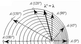
Рис. 3. Картина волн, расходящихся от движущегося вправо источника колебаний. Объективно мы видим, что для точки А (0°) λ ' = λ (1 – β), для точки А (180°) λ ' = λ (1 + β). Вопрос: при каком угле θ можно будет наблюдать равенство λ ' = λ? Может быть, при θ = 90°? Нет, это ошибка, так как величина этого угла явно зависит от значения β и очевидно, что θ > 90°.

Неважно, где находится наблюдатель — рядом с источником, где-то в одной из точек А или смотрит на волновую картину откуда-нибудь сверху — в любом случае он сможет снять зависимость λ ' от угла θ и скорости β:

при θ = 0° ,   λ ' = λ (1 – β) ;         при θ = 180° ,   λ ' = λ (1 + β).

Эти две формулы элементарны и всем известны со школьной скамьи. Трудности вызывал случай равенства длин волн: λ ' = λ. Где, в каком месте представленной здесь картины волн он произойдет?

Традиционно считалось, что этот момент наступит при угле θ = 90°. Но интуитивно каждый понимаем, что значение искомого угла θ зависит от скорости источника колебаний: чем больше скорость β, тем больше линия, где λ ' = λ, отклоняется влево от вертикали (рис. 3), т.е. угол θ становится всё более тупым. Не может получаться так, что скорость β как-то меняется, а угол θ остается постоянно прямым.

Итак, из ранее приводимой формулы:

нам нужно определить, как меняется угол θ в зависимости от скорости β, когда выполняется равенство : λ ' = λ. Если подставить это условие в данную формулу, то найдем простую зависимость :

β   =   – 2 cos θ     или     θ   =   arccos ( – β / 2 ) .

Для наглядности составим нижеследующую таблицу, из которой можно видеть, что любая скорость источника приводит к отклонению луча, для которого λ ' = λ, от вертикальной линии в противоположную сторону от направления движения источника. Данное отклонение является следствием проявления аберрации, хорошо известной физикам. Если β > 0, то θ > 90°. По достижении скорости β = 1, угол отклонения в точности равен θ = 120°.

Таблица скоростей β и углов θ,
сохраняющих условие равенства
длин волн λ ' = λ.

β 0,0001 0,001 0,01 0,1 0,2 0,4 0,6 0,8 1,0 1,2 1,4 1,6 1,8 2,0 2,2

θ 90°,003 90°,03 90°,3 92°,9 95°,7 101°,5 107°,5 113°,6 120°,0 126°,9 134°,4 143°,1 154°,1 180°,0   —

Ничего качественно нового не произойдет, когда скорость звука будет преодолена (рис. 4): β > 1. И только при β ≥ 2 наступает ограничение для выполнения условия λ ' = λ. Скорость источника может быть, конечно, любой, в том числе и β = 2,2 , только воспринимаемая длина волны никогда не будет равна собственной длины волны источника: λ ' ≠ λ.

Рис. 4. Конус ударной волны, образующийся при β > 1. Обратите внимание, здесь нарисованы только левые части окружностей, ограниченные границами конуса ударной волны. Правые участки волновых фронтов не существуют, поскольку волны с отрицательными значениями λ ' в природе отсутствуют.

Что здесь может помешать выполнению условия λ ' = λ ? Разве кто-нибудь отменял выше написанные формулы —

при θ = 0° ,   λ ' = λ (1 – β) ;         при θ = 180° ,   λ ' = λ (1 + β) ?

Да, первая формула для угла θ = 0° здесь отменена. Дело в том, что исходная формула накладывает еще одно ограничение на углы и скорости, а именно: подкоренное выражение всегда должно быть положительным:

1 – β² sin ² θ ≥ 0,     sin θ   ≤   ±1 / β   или   θ   ≤   ± arcsin ( 1 / β ).

Это ограничение дает формулу Маха для нахождения углов внутри конуса ударной волны: sin θ = 1 / β . Пусть β = 2,2 , тогда, согласно последнему ограничению, имеем:

θ   ≤   ± arcsin ( 0,45 )   =   ± 27°.

Это означает, что при β = 2,2 волны не выходят за пределы конуса ударной волны с углами при вершине ±153°, если отсчет вести от положительного направления оси x. Таким образом, при θ = 180° будем иметь λ ' = 3,2 λ, что допустимо, а угол θ = 0° в этой ситуации мы просто не имеем права рассматривать. В этом направлении у нас получилась бы отрицательная длина волны λ ' = –1,2 λ, что с точки зрения физики лишено всякого смысла.

Более того, второе ограничение опережает первое. При любом значении β > 1, когда должны появляться волны с отрицательной длинной,

λ ' = λ (1 – β) < 0,

тут же исчезают правые участки волновых фронтов, распространяющиеся по ходу движения источника колебаний. Вся их колебательная энергия сосредоточивается на границе конуса, что проявляется в виде высокого энергетического барьера.

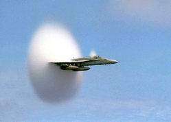
Рис. 5. Фотография реактивного самолета FA-18, летящего быстрее звука. Вблизи летального аппарата виден светлый конус ударной волн. Дело в том, что сразу же за конусом создается зона пониженного давления, в которой происходит мгновенная конденсация паров влаги. В 1911 году Э. Мах установил, что угол θ при вершине конуса ударной волны всецело определяется относительной скоростью β, поэтому параметр β часто называют числом Маха.

Когда реактивный самолет преодолевает этот мощный звуковой барьер (рис. 5), мы слышим оглушительный хлопок. Если бы реально существовали правые участки всех волновых фронтов, то было бы не понятно, откуда конус ударной волны черпает свою колоссальную энергию, т.е. здесь нарушался бы элементарный энергетический баланс. Кроме того, при сохранении правых участков волновых фронтов внутри конуса образовывалась бы интерференционная картина, (рис. 6) которая в действительности не наблюдается.

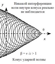
Рис. 6. Показана интерференционная картина, которая в действительности отсутствует. Это означает, что правые участки волн, распространяющиеся в направлении движения источника, реально не существуют. Вся их акустическая энергия в виде сжатого воздуха передается на границу конуса. Таким образом, можно наблюдать только левые участки волн, которые распространяются в направлении отрицательных значений оси x, т.е. против движения источника колебаний.

Все эти нюансы очень важны для осмысления простого математического факта, а именно. Традиционная формула, описывающая плоские волны от движущегося точечного источника колебаний в большинстве случаев не работает даже приближенно, т.е.

λ '  ≠  λ (1 – β cos θ).

Это ложное для сферических волн выражение не описывает всех тех явлений, о которых только что рассказывалось. То есть, традиционная формула не дает наблюдаемые эффекты, отображенные на рис. 2 – 5. Она не отвечает на два важнейших вопроса: 1) откуда берется конус ударной волны; 2) как истолковать отрицательные длины волн λ ' < 0, когда скорость источника превышает скорость звука β > 1. Но все эти факты получают логическое объяснение, если воспользоваться чуть более сложным выражением, справедливым для любых значений β:

.

Если сюда подставить θ = 90°, мы получим выражение, которое в теории относительности получило название поперечного эффекта Доплера. Его суть сводится к уменьшению исходной длины волны λ, генерируемой источником колебаний, до величины λ ' (рис. 7) :

.

Рис. 7. Чертеж иллюстрирует возникновение поперечного эффекта Доплера при β < 1 и θ = 90°

Данный геометрический факт, отображенный на рис. 7, сторонники теории относительности объясняют замедлением времени.

.

Они утверждают, что при θ = 90° выполняется равенство λ' = λ , но за счет «замедления времени» происходит «сокращение длины», так как

λ = c T       и       λ ' = c T '.

Для акустики такая логика не приемлема, так как скорость звука и скорость его источников не попадает в релятивистскую область. С самого начала нужно было отказаться от традиционной формулы и использовать формулу Доплера для сферических волн. Однако жесткие философско-методологические ограничения, господствовавшие в науке XX столетия, не позволили этого сделать. Всё, что грозило подорвать теоретическую базу релятивизма, немедленно изгонялось из сферы науки. Сегодня физическая наука переживает глубокий кризис. Можно надеяться, что с его окончанием физики откажутся от формально-спекулятивной идеологии и снова возьмут на вооружение рационально-конструктивную методологию.

Ошибочные взгляды возникли еще в конце XIX века при постановке и объяснении эксперимента Майкельсона — Морли (1881, 1887). В этом опыте, наделавшем столько шума, использовался источник света конечных размеров, который можно было бы принять за точечный. При поворотах интерферометра на столь значительные углы в нем не возникали условия для плоских волн. Поэтому было бы правильнее считать, что световые волны исходят от локализованного источника, т.е. имеют строго сферическую форму, как это показано на рис. 8.

Рис. 8. Здесь показаны три длины волны: две продольные — λ₁ и λ₂ и одна поперечная — λ₃ , отношение между которыми в точности соответствует отношению между реальными длинами. Помимо этого на рисунке показана еще одна длина волны — λ_3' , которая отвечает за отклоненный в результате аберрации луч 3' .

Между тремя выделенными волнами сферической формы, показанными на этом рисунке, могут располагаться миллионы других волновых сфер: суть дела от этого не меняется, т.е. малая длина волны по сравнению с расстоянием от источника до приемника не делает волны плоскими.

При движении источника происходит отклонение луча 3 на угол α, который откладывается в противоположную сторону по отношению к направлению движения интерферометра, что давало луч 3'. Но Майкельсон, Лоренц и все последующие за ними физики отклоняли луч 3 походу движения интерферометра, что привело к ошибочному анализу хода лучей в интерферометре (рис. 9).

Рис. 9. Майкельсон считал, что луч 1 от источника света 0 распространяется в направлении движения Земли; луч 2 — это отраженный от зеркала С луч 1. Луч 3, отразившись от зеркала А, становится лучом 4. Как отметил Майкельсон, оптический путь, проделанный лучами 1-2, не равен оптическому пути, проделанному лучами 3-4. Следовательно, встретившись в точке В они дадут интерференционные полосы, расстояния между которыми пропорционально разности хода лучей 1-2 и лучей 3-4. В действительности же, никакого луча 3, направленного в точку A, не существует; есть луч 3', направленный под углом α в точку D.

Отрицательный результат опыта объясняется очень просто. Интерферометр Майкельсона, где источник и приёмник установлены на одной платформе, действует компенсационный принцип, нейтрализующий действие эффекта Доплера и явления аберрации. Всё происходит так, как если бы интерферометр никуда не двигался относительно светоносной среды, т.е. не перемещался бы в космосе вокруг Земли и вокруг собственной оси. Поэтому однажды настроенная интерференционная картина, возникшая за счет различной длины горизонтального и вертикального плеча, в процессе движения интерферометра абсолютно бы не менялась (более подробный анализ проведен в разделе Эксперимент Майкельсона – Морли).

Во второй части данной веб-страницы в качестве приложения приводится полный текст английской статьи «Ultrasound Doppler Probing of Flows Transverse with Respect to Beam Axis», в которой экспериментально доказывается существование поперечного эффекта Доплера для ультразвуковой системы, использующейся для выявления патологии сердечно-сосудистой системы. Чтобы уловить главную идею представленной здесь статьи, достаточно прочитать аннотацию к ней. Ниже приводится русский перевод этой аннотации.

«Принято считать, что поперечные эффекты Доплера первого порядка по v/c не существует для всех волновых явлений, включая акустические, т.е. эффект Доплера равен нулю для излучения, направленного перпендикулярно к движению [потока частиц]. Однако такое утверждение предполагает, что падающее поле [ультразвука] представляет собой плоскую волну, что, вообще говоря, не верно для источников с конечной апертурой. Поэтому исследование потоков, перпендикулярных к лучам [ультразвука] конечного диаметра, особенно, когда эти лучи сфокусированы, вполне возможно. Подобная геометрия будет полезна в тех случаях, когда не возможна традиционная ориентация ультразвукового луча вдоль направления потока. Исходя из этих соображений, здесь представлены теоретически и экспериментально выполненные измерения доплеровского спектра для поперечных конфигураций.

Сравнение измерений текущего потока с измерениями, полученными на основе стандартной ультразвуковой Доплер-системы, показывает, что скорость потока, перпендикулярного к оси сфокусированного датчика может быть измерена с точностью, которая сопоставима с точностью, полученной при помощи традиционной системы с наклонной ориентацией [ультразвукового луча]. Измерение Доплер-спектра показывает высокую степень согласованность с теорией.

Хотя эксперименты были проведены для акустических волн, представленные результаты должны быть применимыми также и к электромагнитным системам».

В начале Введения авторы статьи еще раз подчеркивают мысль, выраженную в последнем абзаце аннотации: «Упрощенный эффект Доплера (т.е. для случая плоской волны) применим как к электромагнитным, так и к акустическим волнам. Для цели, двигающейся со скоростью v, точный релятивистский анализ для электромагнитных волн в вакууме производится по той же самой формуле, что и для отраженной частоты   f_s ,   как это делается в акустическом анализе, а именно:

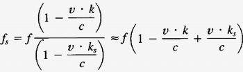,       (1)

где   k, k_s   — единичный вектор в направлении распространения падающего (incident) и отраженного (scattered) возбуждения, соответственно. Понятно, что выражение (1) можно свести к выражению первого порядка [по отношению v/c], которое обычно используют для поперечных волн, т.е. для волн, падающих под прямым углом к движению [частиц], когда   v · k = v · k_s = 0   [ v · k = v cos θ ]   мы получаем   f_s = f ,   что приводит к исчезновению эффекта Доплера. Для случая k_s = – k эффект Доплера удваивается:

f_s = f ( 1 – 2 v · k / c )     [ или   Δ f = 2 f β cos θ ] .     (1а)

Аргумент вблизи направления поперечного движения не заканчивается выражением (1). В релятивистской электродинамике эффекты второго порядка могут быть обнаружены [из-за явления аберрации]. Аргументы такого рода привели к выводу: обнаружение поперечного движения невозможно, особенно в механических системах, в частности, в акустике. Однако, этот довод относится только к плоским падающим волнам бесконечной протяженности, тогда как в действительности мы обычно сталкиваемся с лучами конечной протяженности. Поскольку рассеивание луча размывает плоские волны, которые становятся наклонными относительно оси, или, другими словами, из-за неоднородности возбуждения в поперечном сечении луча, мы могли бы измерить движение, поперечное к оси луча. Еще более сильные эффекты будут наблюдаться при фокусировке лучей, когда в фокальной области наблюдается большой пространственный уклон поля излучения».

Поясним. Выражение (1) эквивалентно ранее приведенной формуле:

,

если принять в ней совпадение углов:   θ₁ = θ₂ = θ ,   равенство по модулю, но разнонаправленность скоростей источника и приёмника:   β = β₂ = – β₁   (что означает   k_s = – k ),   а также пренебречь членами второго и выше порядков по   β = v/c , то оно переходит в выражение   (1а) , откуда находится относительная скорость эритроцитов:

β = ( f ' – f ) / 2 f cos θ .     (1b)

В самом деле, все эти условия выполняются, когда луч ультразвука направлен под небольшим углом наклона к кровеносному сосуду, в котором двигаются частички вещества (эритроциты). Удвоение эффекта Доплера, которое фигурирует в формуле (1а), происходит из-за отражения лучей от всех частиц крови, которые начинают играть роль вторичных источников излучения. Поскольку они двигаются с разной скоростью — у стенок сосуда медленнее и намного быстрее ближе к центру сосуда — то в УЗИ-установке наблюдается широкий спектр принятых частот и, соответственно, Доплер-спектр скоростей представляет собой нормальное распределение.

Формула (1) и ее модификации справедливы только для плоских волн, которые на практике обычно не наблюдаются. Если источник излучения точечный — что ближе к реальности — правильнее было бы воспользоваться другой формулой, которая не использовалась авторами статьи:

.     (2)

Тогда при тех же самых малых углах наклона (θ₁ = θ₂ = θ и k_s = – k ) выражение (1b) заменяется на более подходящее для этого случая:

β = ±( sin² θ + F ² cos² θ ) ^–½ , где F = ( f ' + f ) / ( f ' – f ) .   (2a)

Для поперечного эффекта Доплера имеем более простое выражение:

f ' = ± f (1 – β² ) ^{– ½}   или   β = ±[ 1 – (f ' / f )² ] ^{– ½} ,     (2b)

которое, однако, выполняться будет приблизительно за счет разброса скоростей движения эритроцитов внутри кровеносных сосудов и явления двойной аберрации.

В связи с разбросом скоростей авторы статьи специально подчеркивают, что они исследовали исключительно ламинарные потоки крови, когда все эритроциты движутся пускай и с различной скоростью, но только в одном направлении. Они исключили случай турбулентного движения, при котором частицы перемещаются вперед-назад.

График Fig. 10 (ниже он воспроизведен как рис. 10) наглядно демонстрирует успешность нахождения различных значений скорости кровотока, когда ультразвуковое излучение направлено перпендикулярно к направлению скорости кровотока (θ = 90°). Для сравнения на этом же графике приведены значения скорости для угла θ = 60°, когда используется традиционное приближение (1b) (о формулах 2, 2a и 2b авторы статьи, по-видимому, ничего не знали).

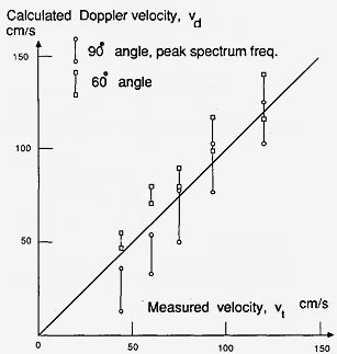
Рис. 10. Сравнение осевой скорости v₁ , полученной непосредственно из расчета по экспериментально измеренным значениям скорости кровотока, с осевой скоростью v_d , полученной по результатам оценки доплеровского спектра.

Итак, зная объемный расход жидкости и площадь сечения трубки, можно вычислить осевую скорость кровотока v₁ . Эксперимент проводился для пяти таких скоростей:

v_1-1 = 43 см/с,
v_1-2 = 60 см/с,
v_1-3 = 74 см/с,
v_1-4 = 93 см/с,
v_1-5 = 121 см/с.

Осевая скорость кровотока v_d , рассчитанная по доплеровским спектрам, находится в доверительных интервалах:

v_{d-1 60°} = 23 ± 12 см/с,       v_{d-1 90°} = 50 ± 4 см/с,
v_{d-2 60°} = 41 ± 10 см/с,       v_{d-2 90°} = 72 ± 5 см/с,
v_{d-3 60°} = 62 ± 13 см/с,       v_{d-3 90°} = 81 ± 5 см/с,
v_{d-4 60°} = 86 ± 10 см/с,       v_{d-4 90°} = 106 ± 7 см/с,
v_{d-5 60°} = 110 ± 11 см/с;       v_{d-5 90°} = 126 ± 12 см/с.

Для угла θ = 60° оценка доплеровской скорости v_d рассчитывалась, исходя из «стандартного уравнения Доплера»:

f_d = 2 f₀ (v/c) cos θ ,

где f₀ — собственная частота излучателя, f_d — доплеровская частота и θ — угол между осью луча и направлением скорости кровотока.

Для угла θ = 90° оценка по всем пяти скоростям v₁ производилась по максимуму спектральной амплитуды, которая определяется выражением (14) и соответствует центральной частоте ( ω' ) треугольного спектра. В диапазоне

ω ( 1 – γ / 2 ) ≤ ω' ≤ ω ( l + γ / 2)

максимум находится в районе

где W — диаметр линзы, F — фокусное расстояние (см. рис. 1 — геометрия поставленной задачи).

Сам спектр, имеющий форму равнобедренного треугольника, можно видеть на рис. 11 (Fig. 4).

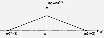
Рис. 11. Спектральные амплитуды, соответствующие заданной ширине линзы W и ее фокусному расстоянию F, а также поперечной скорости кровотока v, достигают максимума на частоте ±ωγ = ±ω (v/c) (W/F).

Для тех, кто далек от медицины и УЗИ-диагностики, дополнительно сообщаем, что патология сердечно-сосудистой системы (например, сужение растворов клапанов сердца или отдельных участков кровеносной системы) определяется по скорости движения эритроцитов. Чем выше их скорость, т.е. параметр β = v/c, тем уже отверстие, через которое они проходят. Большей величине β отвечает и больший доплеровский сдвиг   Δ f = ( f ' – f ) ,   фиксируемый УЗИ-аппаратурой. Как мы знаем, скорость эритроцитов различна в различных точках сечения сосуда. За реальную скорость кровотока обычно принимают скорость движения эритроцитов, движущихся по центральной части сечения сосуда вдоль его оси, где скорость более равномерна и максимальна.

Возможно, что на практике детерминистская формула (2) еще долго не будет играть сколько-нибудь существенной роли, так как ее высокая точность не достижима для статистических измерительных систем с ограниченной фокусировкой луча и конечной апертурой датчика, в которых осуществляется Фурье-анализ. Выражение ( 2b ) дает математически безукоризненную взаимосвязь между скоростью β и частотным сдвигом Δ f при θ = 90° — другой формулы просто не может быть. Главным же в ультразвуковой диагностики оказывается наличие самого факта поперечного эффекта Доплера, который возникает не в результате эфемерного замедления времени, как учат нас релятивисты, а за счет искривления волнового фронта или, иначе сказать, отсутствия условий для существования идеальных плоских волн.

Напомним, что скорость ультразвука, распространяющегося в биологическом организме, равна приблизительно c = 1540 м/с ; максимальная скорость перемещения эритроцитов на три порядка меньше — v = 1,5 м/с. Таким образом, в процессе ультразвуковой диагностики отсутствуют условия для проявления релятивистских эффектов, к которым относится поперечный эффект Доплера, тем не менее, он регистрируется медицинскими приборами. При β = 0,001 и частоте излучения f = 10 МГц , приёмник зафиксирует частоту f ' на 5 Гц ниже, чем у излучателя.

Теперь, наконец, желающие ознакомиться поближе с использованием в медицине поперечного эффекта Доплера могут приступить к чтению второй части данного раздела, где приведен полный текст вышеупомянутой статьи на английском языке. Заметим только, что приведенной ниже статье предшествовал развернутый доклад [1], сделанный двумя основными авторами статьи (Dan Censor and Vernon L. Newhouse). На симпозиуме 1986 года они представили более детальные математические выкладки, которые не вошли в их статью 1987 года. Начинали же они еще в 1960-х годах и продолжали работать в течение нескольких десятилетий (посмотрите, например, их статью 1994 года [2]). В статье 2002 года [3] двумя другими авторами сделан обзор различных методик ультразвуковой диагностики, связанный с эффектом Доплера, в том числе, поперечным. Этот обзор основывается на списке источников, которым мы завершим первую часть данной веб-страницы.

---

1. D. Censor and V. L. Newhouse. Theory Of Ultrasound Doppler-Spectra Velocimetry For Arbitrary Beam And Flow Configurations. IEEE 1986 Ultrasonic Symposium, pp. 923-932.
2. Newhouse,V.L., Censor,D.,Vontz, T. et al., Ultrasound Doppler probing of flow estimation using two transducers and spectral width, IEEE Trans. Ultrason. Ferroelect. Freq. Contr. 41, 90-95 (1994).
3. Chih-Kuang Yeh and Pai-Chi Li. Doppler Angle Estimation of Pulsatile Flows Using AR Modeling. Ultrasonic Imaging 24, 135- 146 (2002).
4. Jensen, J.A., A new estimator for vector velocity estimation, IEEE Trans. Ultrason. Ferroelect. Freq. Contr. 48, 886-894 (2001).
5. Anderson, M.E., Multi-dimensional velocity estimation with ultrasound using spatial quadrature, IEEE Trans. Ultrason. Ferroelect. Freq. Contr. 45, 852-861 (1998).
6. Bohs, L. N., Friemel, B. H. and Trahey, G. E., Experimental velocity profiles and volumetric flow via two-dimensional speckle tracking, Ultrasound Med. Biol. 21, 885-898 (1995). 7. Bohs, L. N., Geiman B. J. AndersonM. E. et al., Ensemble tracking for 2D vector velocity measurement: experimental and initial clinical results, IEEE Trans. Ultrason. Ferroelect. Freq. Contr. 45, 912-924 (1998). 8. Tortoli P., Guidi G., Mariotti V. and Newhouse, V.L., Experimental proof of Doppler bandwidth invariance, IEEE Trans. Ultrason. Ferroelect. Freq. Contr. 39, 196-203 (1992).
9. Tortoli P., Guidi G. and Newhouse V.L., Improved blood velocity estimation using the maximum Doppler frequency, Ultrasound Med. Biol. 21, 527-532 (1995).
10. Lee B.R., Chiang, H.K., Chou, Y. H., et al., Implementation of spectral width Doppler in pulsatile flow measurements, Ultrasound Med. Biol. 25, 1221-1227 (1999).
11. Li, P.C., Cheng, C.J. and Shen, C.C., Doppler angle estimation using correlation. IEEE Trans. Ultrason. Ferroelect. Freq. Contr. 47, 188-196 (2000).
12. Yeh, C.K. and Li, P.C., Doppler angle estimation using AR modeling, IEEE Trans. Ultrason. Ferroelect. Freq. Contr. 49, 683-692 (2002).
13. Kay, S.M., Modern spectral estimation: Theory and application (Englewood Cliffs, NJ: Prentice Hall, 1988).
14. Kerr, A.T. and Hunt, J W., A method for computer simulation of ultrasound Doppler color flow images-I. Theory and numerical method, Ultrasound Med. Biol. 18, 861-872 (1992).
15. Evans, D.H., Some aspects of the relationship between instantaneous volumetric blood flow and continuous wave Doppler ultrasound recordings III, Ultrasound Med. Biol. 9, 617-623 (1982).
16. Jensen, J.A. Estimation of blood velocity using ultrasound: A signal processing approach (New York: Cambridge University Press, 1996).
17. Marasek, K. and Nowicki, A., Comparison of the performance of 3maximumDoppler frequency estimators coupled with different spectral estimation methods, Ultrasound Med. Biol. 20, 629-638 (1994).
18. Bascom, P.A. J., Cobbold, R. S. C., Routh, H. F. et al., On the Doppler signal from a steady flow asymmetrical stenosis model: effects of turbulence, Ultrasound Med. Biol. 19, 197-210 (1993).
19. Cloutier, G., Chen, D. and Durand L.-G., Performance of time-frequency representation techniques to measure blood flow turbulence with pulsed-wave Doppler ultrasound. Ultrasound Med. Biol. 27, 535-550 (2001).
20. Schlindwein, F. S. and Evans, D. H., A real-time autoregressive spectrum analyzer for Doppler ultrasound signals, Ultrasound Med. Biol. 15, 263–272 (1989).
21. Hein, I.,A., 3-D flowvelocity vector estimationwith a triple-beamlens transducer experimental results, IEEE Trans. Ultrason. Ferroelect. Freq. Contr. 44, 85-89 (1997).

IEEE TRANSACTIONS ON BIOMEDICAL ENGINEERING,
VOL. BME-34, No. 10, OCTOBER 1987, pp. 779 – 789

Ultrasound Doppler Probing of Flows
Transverse with Respect to Beam Axis

VERNON L. NEWHOUSE, FELLOW, IEEE, DAN CENSOR, THOMAS VONTZ,
JOSE A. CISNEROS, AND BARRY B. GOLDBERG

Abstract. It is an accepted fact that transverse Doppler effects of the first order in v/c are nonexistent for all physical wave phenomena, including acoustics, i.e., the Doppler effect is zero for radiation normal to the direction of motion. However, this statement assumes that the incident field is a plane wave, which is not true in general for finite aperture sources. Consequently, the probing of flows transverse to the axis of finite diameter beams, particularly focused beams, is feasible. This geometry will be advantageous in many applications where the classical orientation of the sound beam, oblique to the flow, is not possible. With this motivation in mind, the theory and experimental feasibility of measuring Doppler spectra in transverse geometries is presently investigated.

The comparison of flow flux measurements, and measurements performed using a standard ultrasound pulsed Doppler system, show that flow normal to the axis of a focused transducer, can be measured with an accuracy comparable to that obtained with the conventional oblique orientation. The measured Doppler spectra are shown to agree well with theory.

Although the experiments have been performed for acoustical waves, the present results should also be applicable to electromagnetic systems.

INTRODUCTION

The simplistic (in the sense of incident plane wave) Doppler effect [1]-[3] has been applied to electromagnetic as well as acoustical waves. For a target with velocity v, the exact relativistic analysis for electromagnetic waves [2], [4], [5] in vacuum yields the same formula for the scattered frequency f_s as does the acoustic analysis, namely.

,       (1)

where k, k_s, is a unit vector in the direction of propagation of the incident, and the scattered field, respectively. Clearly, (1) reduces to the first-order expression commonly used, and demonstrates that for transverse waves, i.e., for waves at right angles to the motion where v · k = v · k_s = 0, we obtain f_s = f and the Doppler effect vanishes [6]. For k_s = –k, the Doppler effect is doubled

f_s = f (1 – 2v · k/c).       (1а)

The argument about the direction of transverse motion does not end with (1). In relativistic electrodynamics, second-order effects due to the aberration phenomenon may be detectable [7], [8]. Arguments of this kind led to a concensus that the detection of transverse motion, especially in mechanical systems, e.g., acoustics, is impossible However, this argument only applies to incident plane waves of infinite extent, whereas in real life, we usually encounter beams of finite width. Because the decomposition of the beam field involves plane waves which are oblique with respect to the axis, or in other words, due to the inhomogeneous field in the cross section of the beam, we might still be able to measure motion transverse to the beam axis. Even stronger effects should be obtainable with focused beams where the spatial gradient of the field is large in the focal region. In an earlier study [9] based on geometrical ray arguments, it has been shown that the breadth of the Doppler output spectrum was dependent on the angles made by the outer rays of the illuminating sound beam with the flow direction. In the present study, using a more rigorous diffraction theory, this result is shown to hold true even when the flow direction is at right angles to the beam axis. Note that the results of the present paper which demonstrate that Doppler signals are produced by laminar flow normal to the axis of a focused transducer, should not be confused with recent studies [10], [11] in which transducers oriented at right angles to blood vessels are used to obtain Doppler signals from vortexes. In that case, the Doppler signals result mainly from the flow components which are not normal to the beam axis.

The present study is anchored by the experimental work of Cisneros [12], for which a theoretical model is devised and analyzed. The first geometry analyzed is that of a two-dimensional strip transducer. This provides results which can be interpreted in terms of geometrical or ray acoustics and used to qualitatively explain our experimental results [13]. This is followed by a more complex analysis of the more realistic case of a cylindrical transducer which gives results in quantitative agreement with experiment.

The theory given below shows that the echo amplitude spectral density (i.e., the square root of the power spectral density) expected from a two-dimensional long strip aperture beam, focused on particles moving with velocity v normal to the beam direction, has a triangular shape. The peak of this spectrum (shown in Fig. 4) is at ω = 2πf where f is the transmitted frequency, and the extrema are at ω[1 ± γ] = ω[1 ± (v/c) (W/F)] where W is the width of the transducer and the focal length F >> W.

The experiments reported here [12] used a circular aperture transducer, for which our theory predicts an echo spectrum of the same bandwidth, but having the shape of a "rounded" triangle, shown in Fig. 7, again centered on the (angular) frequency ω. The experimental results agree with the numerical results based on theory, within the accuracy expected from the approximations that were made. Note also that Bascom et al. [14] have recently numerically computed a spectrum of similar symmetry and shape for the case of a continuous Doppler system irradiating transverse flow in the near field of a circular aperture.

The effects reported here, namely the ability to make Doppler flow measurements of flow normal to the beam axis, are of first order in v/c and are therefore significant for other branches of wave physics, e.g., electromagnetic waves, in similar configurations.

TWO-DIMENSIONAL ANALYSIS

As explained above, the simplest model of the problem which provides physical insight, involves a strip transducer   –∞ < η <+∞   defined at   z = 0   and   –W/2 < ξ < W/2   (see Fig. 1).

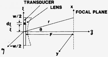
Fig. 1. Geometry of the problem.

For harmonic waves, any acoustical field parameter (the acoustical pressure, say) must satisfy the Helmholtz wave equation.

,       (2)

where c is the speed of sound. Consider a line source element dξ;   –∞ < η < +∞   producing at large distances a field which is omnidirectional in the xz plane

      (3)

This is the asymptotic solution of (2) in the far field kp >> 1 with a proportionality factor K, and

      (4)

(see Fig. 1). The total field produced by the transducer is, [16]:

      (5)

where K is a constant of proportionality and sinc A = (sin A ) / A. Due to the presence of the converging lens in front of the transducer (Fig. 1), all rays at a given angle θ converge at a point x in the focal plane. This justifies the use of the above far field forms for the geometry of a focused transducer. Neglecting lens end effects (vignetting) and assuming that the dimensions of the region of interest in the focal plane are small compared to the focal length F, we have a transformation (see Fig. 2)

sin θ ≈ θ ≈ x/F       (6)

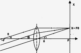
Fig. 2. Transformation of ray angles into distance in the focal plane.

It follows that (5) is approximately given by

      (7)

where r = F in (5), and other terms are absorbed into the new constant K'.

We consider now a stream of scatterers moving in the focal plane with velocity v in the x direction. These small, three-dimensional particles move through the line focus x = 0, z = F, and arbitrary y. Since the transducer (now acting as receiver) is infinite in the y direction, its response to scattering from a point particle, after integration from y = –∞ to y = +∞, is independent of y. Inasmuch as the coordinate y of the particles is irrelevant, we may assume, without lack of generality, that particles are continuously distributed along the y direction. In other words, the situation is equivalent to having thin line "particles" aligned in the y direction. These two-dimensional line particles constitute omnidirectional monopole scatterers radiating in the far field according to

      (8)

where a₀(k' ) is a coefficient depending on the excitation frequency ω', and r' is the distance from the monopole. The line particle is moving according to

x = vt       (9)

where the time origin has been arbitrarily chosen as t = 0. Hence, the excitation field is given by (9) substituted into (7):

      (10)

with γ = (v/c) (W/F). Here we have again substituted r' = F, and the integrand of (10) also displays the spectrum (i.e., the Fourier transform) of the excitation field depicted in Fig. 3; here K" is another constant factor. Note that the boundaries of the spectrum of (10), as shown by the limits of the integral, are identical to the Doppler shifts of the rays emanating from the edges of the transducer and received by a scatterer moving through the focus z = F,   x = 0 at velocity v along the x axis. For example, the rays emanating from the transducer edges ξ = ±W/2 produce Doppler shifts ±ωγ/2 = ±(ω v/c) cos α, where α is the angle subtended by the velocity v and these rays. From (8) and (10) the back-scattered field reaching the transducer (now operating as receiver) at z = 0, is given by

      (11)

where t' = t – F/c is the retarded time and K" is the same factor as in (10). This spectrum is identical to (10), provided a₀(k' ) in the band ω(1 – γ/2) ≤ ω' ≤ ω(l + γ/2) is well approximated by a constant a₀(k ) at the central frequency.

We are now interested in computing the total field intercepted by the receiver. There are two equivalent methods to approach this problem. The more obvious is to say that since we have demonstrated that an argument based on diffraction of waves leads to (10), but since this result could also be reached by computing the Doppler effects due to rays coming from various directions, therefore we are free to use a ray argument to compute the cumulative response of all parts of the receiver [13]. A more general way of looking at the problem is by invoking the principle of reciprocity. This states that if a single frequency at the transducer (acting as transmitter) excites a moving scatterer going through the focus according to the spectrum of (10) and Fig. 3, then this object, if acting as a transmitter at frequency ω', will produce the same spectrum at the extended receiver. In other words, a moving source emitting a frequency ω', passing through the sine function radiation pattern lobes of the receiving transducer, produces an amplitude modulated response in the receiver, having exactly the rectangular spectrum of Fig. 3.

Fig. 3. Shape of amplitude spectral density function for the field exciting the particles moving through the focus. This is also the spectrum received at the center of the transducer (now acting as receiver) due to a moving line particle transmitting at a single frequency ω'.

Thus, we obtain

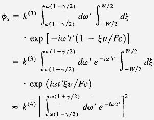      (12)

where   k ⁽³⁾, k ⁽⁴⁾   are new constants,   ξv/Fc = k_s · v/c   according to (1), and we have approximated   ω' = ω   in the second integral because the exponent is already of first order in v/c and only first-order effects in v/c are significant. The two integrals are now independent. The pressure   ф_s   (12), is seen to be proportional to

      (13)

The amplitude spectrum corresponding to this time domain waveform is obtained by convolving the spectrum of Fig. 3 with itself and has a triangular shape as shown in Fig. 4, with extremal Doppler frequency shifts of

      (14)

In continuous Doppler systems, the echo is multiplied by the reference frequency and low-pass filtered, which has the effect of down-shifting it so that the system output echo has the same triangular shaped spectrum, but now centered on zero frequency.

Fig. 4. Amplitude spectrum corresponding to (13) of the signal obtained by a strip transducer of infinite length, width W, and focal length F, observing a transverse flow of velocity v, γ = (v/c)(W/F).

The above analysis was for a single particle, (whether point or line particle). The contributions from many particles, having arbitrary time origins   t₀ , instead of   t₀ = 0   as in (9), add incoherently. This means that we have to add the ordinates of the corresponding power spectral density function. Since the power spectral density function is identical for all particles, it follows that the total echo amplitude spectrum (obtained by taking the square root of the combined power spectral density function) again has the triangular shape of Fig. 4. The same is true for the system output spectrum. Note that if the scatterers passing through the focus exhibit a range of velocities, the spectrum will lose its triangular shape, but (14) will still be valid for the extremal frequencies provided that v is now interpreted as the maximum particle velocity.

THREE-DIMENSIONAL CONSIDERATIONS

The above calculations were performed for an idealized infinite strip transducer, with the justification that this geometry leads to simple results and can be approximated by finite length strip transducers. We now consider the mathematically more complex, but physically more realistic case of the uniform circular aperture transducer. This three-dimensional geometry, involving a uniform circular aperture of radius b₀ , produces the field (see Fig. 5).

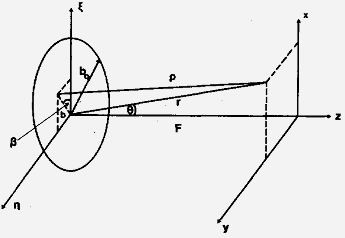
Fig. 5. Geometry of the circular aperture transducer.




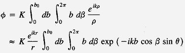
      (15)

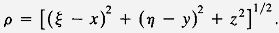
For an arbitrary point x,у we should have in (15) cos (β – φ) where tg φ = y/x (see Fig. 5). Here

ρ = (r ² – 2br cos β sin θ) ^½ ≈ r – b cos β sin θ

has been chosen for a point y = 0 in the focal plane. Because of the circular symmetry of the problem the choice of φ = 0 does not affect the generality of the argument. From (15) we obtain the Fourier transform of the aperture function (i.e., the Fraunhofer approximation) [17], [18]

      (16)

where J₁ is the nonsingular Bessel function of the first order and

      (17)

into which the velocity in the x direction has been substituted. For r = F, the focal distance, and K' absorbing all extra terms, we have the field exciting the particles given by

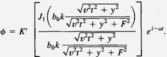      (18)

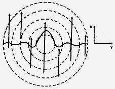
Fig. 6. Sketch of the field in the focal region of the circular aperture transducer. Dashed circles denote zero pressure, arrows denote particle trajectories.

Obviously, the field exciting a particle depends on its off center distance y from the beam axis x = 0, y = 0. (See sketch of field in Fig. 6.) Clearly, a particle moving off the beam axis at large y will go through less pronounced modulation of the field. Consequently, the spectrum associated with this particle, as well as the spectrum produced at the receiver due to this particle, has a narrower profile. This will not affect the edges of the spectrum, Fig. 4, but will cause a peaking of the profile at the central frequency ω. The expression in brackets in (18) corresponds to sinc (ωWvt / 2cF) in (10). The spectrum associated with (18) is obtained by integrating from –∞ to +∞ with respect to t, which corresponds to a Fourier integral. This is indicated by , i.e., we obtain

      (19)

By the argument given above, based on reciprocity considerations, the spectrum received at the extended transducer is obtained by convolving (19) with itself. This is a function of frequency ω', and y, the off-center distance. Finally, we have to add the power spectral densities, i.e., square and integral over all y. The amplitude spectral density function corresponding to the voltage obtained at the output of the receiver is given by the square root, i.e.,

      (20)

The expressions (19), (20) have been numerically evaluated using the following parameters:

W = 2b₀ = 0.01 m,
v = 0.5 m/s,
F = 0.02 m,
ω₀ = 5.0 MHz,
c = 1540 m/s.

Fig. 7(a) shows the resulting exciting beam intensity seen by scatterers with different offsets from the beam axis, i.e., the square of the expression in brackets in (18) for different y values. Fig. 7(b) are the Fourier transforms of Fig. 7(a) corresponding to the echo spectra due to scatterers having specified offsets, that is (19) convolved with itself, for different y values. It can be seen that the contributions of particle trajectories outside the main lobe (in this example, y₄ and y₅ ) are very small, so that later on, the integration will extend over a few Fresnel zones only. Neglecting higher zones does not produce significant errors. Note that the maximal bandwidth is received only for particles passing through the beam center, trajectories with a larger offset produce narrower spectra.

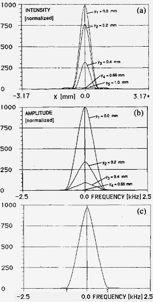
Fig. 7. Amplitude spectra for circular aperture, numerical calculation, (a) Beam intensity [i.e., the square of the term in brackets in (18)] for different y values, seen by scatterers moving at various offsets from the beam axis, (b) Fourier transforms of Fig. 7(a) corresponding to the echo spectra for the different scatterer offsets, (c) Amplitude spectrum for a circular aperture transducer, insonifying uniformly distributed scatterers moving in the focal plane. The arrows indicate the extremal frequencies given by (14).

The final result, namely the calculated spectrum for a circular transducer (20) insonifying uniformly distributed scatterers moving on a plane through the focus, is presented in Fig. 7(c). Numerical integration was performed over the first five Fresnel zones. The extremal frequencies, which should be identical to the corresponding case as derived above for the infinite strip transducer using (15) (± ω₀ (v/c)(W/F) = ±811 Hz), are indicated by arrows. The nonvanishing of the spectrum slightly outside ±811 Hz is probably due to computational errors Since all functions must be calculated for discrete parameter increments, they appear for the computer program as having a staircase pattern instead of a smooth curve. Consequently, the Fourier transform yields for this pattern additional high-frequency components. We expect that noise in a real system will have somewhat the same effect, causing some blurring of the extremal frequencies and rounding the theoretical sharp spectrum edges. This introduces difficulties in determining the edge frequencies (see experimental results). As mentioned above, Bascom, Cobbold, and Roelofs [14] recently derived results based on geometrical considerations and computer simulation. Their results are in agreement with our conclusions.

EXPERIMENTAL PROCEDURES

Experiments designed to verify the theory using commercially available equipment were performed [12], observing continuous and pulsatile flows. The flow model preparation consisted of a plastic tank containing a semirigid plastic tube with an internal diameter of 7.9 mm, i.e., a cross-sectional area of 0.49 cm² and 1.5 m long. This was connected to a plastic reservoir containing 3 1 of blood-simulating mixture of water and glycerol, seeded with chromatography cellulose powder. Flow passed through the tube from an upper to a lower reservoir, with a pump being used to return the fluid to the upper reservoir, thus maintaining a constant fluid level in the top reservoir. For continuous flow, the flow rate was regulated by changing the height of the top reservoir. Timed volume measurements were performed in order to calibrate the flow rate as a function of the height of the top reservoir. From this the average velocity has been computed. For pulsatile flow experiments, a latex tube having the same internal diameter and length was used. A Harvard instruments pump was connected between the top reservoir and the water tank. This pump operated in a pulsatile pattern, and was adjusted to generate waveforms similar to those in the common carotid.

The flow of blood simulating mixtures through plastic tubes was probed by means of a standard ultrasonic medical "Duplex" system which could be switched from imaging to Doppler velocity measurement without changing the transducer position. The Duplex instrumentation consisted of a Technieare Auto Sector which had a built-in spectrum analyzer. This was operated with a mechanical rotating transducer assembly (probe model 1106D) containing three transducer elements, one of them a Doppler optimized single crystal element. Imaging was performed with 7.5 MHz, image optimized single crystal transducer elements in a rotating assembly designed for real-time sectoral imaging. Doppler signals were obtained in the pulsed mode, using a repetition frequency of 15 kHz. The Doppler transducer had a crystal diameter of 11 mm and, according to the manufacturer's specifications, a beam entrance diameter of 8.5 mm. The center frequency of the transducer with 4.55 MHz, with a percent bandwidth of 20 percent, and a range cell of 1 mm length. The focal distance F of the transducer was 22 mm and at this location the beam width was 1.7 mm, which constitutes the lateral dimensions of the range cell.

The high-pass filter of the spectrum analyzer of the Duplex system had a cutoff frequency of 60 Hz. This analyzer had a 60 Hz update rate, taking 128 samples for directional analysis of the Doppler signals. The Duplex system could provide displays of the power spectra, that is, of the frequency versus the power. Typical individual power spectra for pulsatile flow through a rigid tube are shown in Figs. 8 (a) and (b) for beam angles of 60° and 90°, respectively, relative to the flow direction. Note the upper left-hand portion of these pictures, displaying a B-mode image of the flow tube, with the direction of the sound beam indicated by a line. These images were used to orient the transducer beam at right angles to the tube wall, and thus also to the flow. Displays of frequency spectra versus time, with frequency vertical, time horizontal, and with the spectrum amplitude represented by a grey-scale, are shown at the bottom of these two figures, for pulsatile flow having approximately one cycle/s. Two modes of displaying spectra are shown in the top right-hand corners of the figures Fig. 8(a) shows several superimposed spectra each of which is composed of a series of dots, for that portion of the flow cycle corresponding to the right-hand edge of the bottom temporal spectral display. The top right-hand corner of Fig. 8(b) shows a single spectrum for flow receding from the transducer, in which the sample points are connected by lines. The time of this spectrum corresponds to the vertical line in the bottom display.

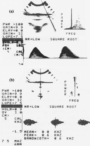
Fig. 8. B-mode flow tube images, individual amplitude spectra, and flow displays for pulsatile flow of approximately one pulse/s. (a) Beam angle at 60° to flow (b) Beam angle at 90° lo flow.

For experiments comparing transverse and oblique flow measurement to time-volume measurements we used the ability of the spectrum analyzer to display graphically and numerically the "peak frequency" of the individual spectra, defined as that frequency which includes 95 percent of the signal power. The graphical display of the individual peak frequencies was used to display pulsatile flow velocities normal to the sound beam, as will be discussed in connection with Fig. 11 below The numerical display of the individual peak frequencies was used to estimate the velocity of continuous flow normal to the sound beam as discussed in the next section in connection with Fig, 10. The peak frequency estimates produced by our Duplex system are dependent on the setting of an amplitude threshold control which is designed to eliminate system noise. Thus, if this threshold is set too low, the peak frequency estimates will be too high or vice versa. For the present experiments, we used the machine preset level. The spectrum analyzer could also calculate and display the mean frequency of each individual spectrum. These frequencies were used to calculate the average range cell velocity from spectra obtained using traditional beam-to-flow angles of less than 90°.

Another set of experiments was performed to examine the degree of agreement between the theoretically predicted spectrum shape [Fig. 7(c)] and the actual spectrum shape [Fig. 9(a)] Because there is a large variance in the individual spectra, these had first to be time averaged to be able to compare them to theory.

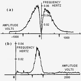
Fig. 9. Experimental amplitude spectra, time-averaged with the Data-6000 waveform analyzer, for a flow velocity of 30 cm/s. Averaging was performed by adding up 100 successive spectra which corresponds to a 10.24 s time period signal (each spectrum was formed from 512, 8-bit samples at 200 μs intervals), (a) Transducer beam axis nearly normal to flow direction, (b) Beam angle at 60° to flow. The arrows in this figure denote the theoretically (for single velocity!) calculated extremal frequencies.

This was accomplished by using a separate programmable waveform analyzer (Data-6000, Data Precision), instead of the nonadjustable spectrum analyzer of the Duplex scanner, to perform Fourier transformation of the Doppler output time-signals and to do spectrum-averaging. These time-signals were provided by the two channel audio-output of the Doppler unit, corresponding to "forward" and "reverse" flow. They were recorded on a high-fidelity VCR before processing with the Data-6000. A comparison between the spectra obtained by using either the actual or the recorded signal showed no observeable difference. Thus, we are confident that the recording fidelity was satisfactory.

By choosing the appropriate time-base and number of sample-points we achieved a much better spectral resolution for the transverse Doppler signals whose frequencies are normally below 1 kHz than would have been obtained with the built-in analyzer of the Duplex system. The latter is designed to be fast and therefore delivers only a few spectrum points in the frequency range below 1 kHz.

Averaging was performed by adding up 100 successive spectra which corresponds to a 10.24 s time period signal (each spectrum was formed from 512, 8 bit samples at 200 μs. intervals. Each channel signal was analyzed separately, resulting in two 256 point spectra which were then combined into the final spectrum, consisting of 512 points.

EXPERIMENTAL RESULTS

Experiments were performed to verify the theoretically predicted transverse flow spectrum shape and to investigate the feasibility of using the spectral width for measuring continuous and pulsatile flows. It has been shown above that for an infinite strip transducer the expected shape for the amplitude spectrum is triangular, and that the extremal Doppler shifts are ±ω(v/c)(W/F). Furthermore, the same extremal frequencies were shown to occur for a circular transducer of diameter W.

Experimental spectra for continuous flow taken with the 1 mm range cell on the axis of the flow tube are shown in Fig. 9. These have been time-averaged with the Data-6000 waveform analyzer and their shapes verify the theoretical predictions of Fig. 7(c) for single velocity flow insonified by a circular aperture transducer, in so far as they exhibit a similar shape, although riding on a "noise pedestal" due to system noise. (Since both the spectrum and system noise are uncorrelated processes, the Doppler and noise spectrum power are additive.) The extremal frequencies predicted by (14) are shown by arrows. These are a little closer together than the apparent width of the spectrum, which may be due to spectral broadening effects that will be discussed in a later paper. The indentation near zero frequency is due to the effect of the wall filter. Fig. 9(b) shows a spectrum for oblique incidence where no wall filter effect occurs and that shape is a "nice" triangle as expected. The derivation for the calculation of the bandwidth for this kind of spectra will be presented in a later paper. The arrows in this figure denote the theoretically (for single velocity!) calculated extremal frequencies.

When comparing the extremal frequencies of the averaged spectra to theory, we have to expect the same uncertainty caused by the arbitrary setting of the noise rejection threshold as those encountered in connection with the peak frequency estimator of the Duplex system. That is, the noise threshold of the estimator has to be set manually above the noise-level, i.e., for poor SNR it may not be clear whether the true highest frequency already lies in the noise region of the spectrum and the estimated peak-frequency is or is not too low. For the averaged spectra, the peak-frequency was determined in two ways:

a) The noise-level was estimated by inspection and the frequency with an amplitude above this level was chosen as "peak."
b) The averaged spectrum was fitted to the nearly triangular shape expected from theory and the crossing over of the triangle side on the frequency axis was used as peak These estimated peak frequencies ranged from about 20 percent to 30 percent above those calculated by (14). In general, our experiments showed that even for arbitrarily chosen noise rejection thresholds, the bandwidth is proportional to the flow velocity.

Fig. 10. Comparison of axial velocity v₁ derived from timed volume experiments with the Doppler estimated axial velocity v_d.

The fact that the shape and width of our averaged spectra agree with theory does not however guarantee that the bandwidth of unaveraged spectra can be estimated accurately and rapidly enough by the Duplex maximum frequency estimator for the results to be clinically useful. To test this estimator circuit, Doppler spectra for continuous flow were measured with both 90° and 60° beam-to-flow angles, using the instrumentation described above. For these experiments the measurement volumes were placed on the axis of the flow vessel, and far enough from the entry port, so that the velocity profile could be assumed to be parabolic. Under these circumstances, the maximum velocity within the range cell will be the axial velocity which is known to equal twice the average flow velocity. The average flow velocity for these experiments was determined, as mentioned above, by measuring the quantity of fluid passing through the tube in a known time. For each of five different velocities, using the 90° orientation, three to seven different values of the "peak" spectral frequency were measured using the built in spectral analyzer. The velocities calculated from these frequencies using (14) are plotted against the axial velocity calculated from the mechanically measured average velocity in Fig. 10. Using the classical 60° transducer orientation, the spectrum analyzer was used to calculate the mean spectral frequency, for three to seven individual spectra taken at each of the five velocities used in the 90° experiments. From these mean frequencies, the corresponding tube axial velocities were calculated using the standard Doppler equation

f_d = 2 f₀ (v/c) cos θ

[i.e., (1a) approximated to first order in v/c ] where θ is the angle between the beam axis and the flow velocity, and f₀ and f_d are respectively the transmitted frequency and the Doppler output frequency f₀ and f_d . These "60 degree" Doppler velocities are also plotted in Fig. 10 against the axial velocities calculated from the mechanically measured flows. Examination of this figure shows that the velocities estimated from the extremal frequencies of the 90° orientation spectra are nearly as accurate as those estimated from the mean frequencies of the 60° orientation spectra. It appears that the scatter of the 90° extremal frequencies are somewhat worse than that of the 60° orientation mean frequencies.

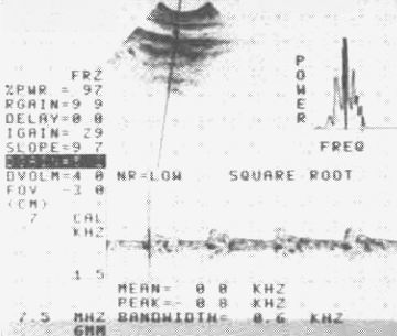
Fig. 11. B-mode image, individual spectrum, and pulsed flow display for a common carotis with a tracing computed with the maximum frequency estimator circult of the Technicare system. Transducer beam axis nearly normal to flow direction.

Using the maximum frequency display of the Technicare system, it was possible to display the axial velocity for pulsed flow, using the 90° beam-flow orientation. However, for moderate pulsatile flow velocities, it was found that the Technicare system could only display the waveform during the "systolic" part of the pump cycle, since the Doppler shifts produced during the "diastole" when the pump delivered constant velocity flow, were too low for the system to process and display. Presumably, this was due to the high-pass filter cutoff occurring at 60 Hz. (The wall Doppler echo rejection filters of the Duplex system had been turned off for these experiments.) In vivo pulsatile flow displays of the common carotis, computed with the "maximum frequency" estimator of the Technicare system are shown in Fig. 11. This picture is included to demonstrate the different effects caused by axial and radial flow with a 90° or near 90° angle between die beam and flow axes. The positive and negative axes of this display represent approaching and receding flow directions, respectively. For axial pulsatile flow normal to the beam, the maximum frequency tracings are roughly symmetrical with respect to the horizontal time axis.

SUMMARY AND DISCUSSION

This paper has calculated theoretically that pulsed directional Doppler systems emitting focused beams normal to the direction of a flow produce simultaneous symmetrical "approaching flow" and "receding flow" Doppler spectra which peak at zero frequency and whose extremal frequencies are proportional to the maximum velocity in the range cell which is assumed to coincide with the beam focus. The theory predicted a slightly rounded triangular shape for the spectrum produced by a circular aperture transducer with the spectral bandwidth

      (21)

Note that this bandwidth calculated here using diffraction theory, agrees closely with that calculated for arbitrary beam-to-flow angles using the ray approximation [9].

With a waveform analyzer and averaging techniques, we compared experimental and calculated spectral shape, finding good agreement. The discrepancies are believed to be due to bubble noise and finite bandwidth effects which will be considered in the future.

Note also that the spectral bandwidth of the Doppler system output signal and of the received echo are the same, and that the inverse of this bandwidth corresponds to the width τ of the autocorrelation function of these signals. Thus, we can define a signal coherence time τ using the distance between the zeros of the main lobe of the sinc² function (13), i.e., ( čWvτ )/(2cF ) = 2Ą. This yields

,       (22)

which is naturally of the same order of magnitude as и 1/Δf. From (7), we see that the coherence time is approximately equal to the scatterer transit time across the beam focus. Since for time intervals greater than the coherence time, the echo and output signals lose coherence, we see that τ also equals the average time between zero crossings of the output Doppler signals. Thus, instead of using the spectral bandwidth of the output signal to estimate velocity, one could have used its average zero-crossing interval. Alternatively, we could have used the average time interval at which the envelope of the echo crosses its mean value which can also be seen to be equal to τ. This latter method was in fact demonstrated by Atkinson [19], [20]. Atkinson viewed his technique as estimating velocity through the "fading rate" of the fluid echo, and derived an expression for the echo coherence time essentially identical to (22), except for a numerical constant. From this point of view, our methods are equivalent, but the spectral properties of the Doppler signal contains additional information, and also provides a convenient transition to the estimation of nontransverse flows. This is illustrated by Fig. 8(a) where the spectrum analysis method is seen to be usable for both transverse and non-transverse flow estimation.

This paper has also shown that with a commercially available Duplex system insonifying continuous flow through rigid tubes, it is possible, using the maximum frequencies of the obtained spectra, to estimate the flow velocity with an accuracy similar to that obtained when the flow velocity is estimated with the traditional Doppler acute angle beam-to-flow orientation. By displaying the continuously calculated "maximum frequency" of the 90° orientation spectra it was found possible to track pulsatile flow velocities, although lower velocity portions of the flow cycle might be unobservable due to the 60 Hz filter of the Duplex system.

The results of this paper, summarized above, show that real time Doppler flow measurements are possible even when the sound beam is at right angles to the flow direction, and that the maximum velocity in the range cell can be calculated from the maximum frequency of the spectrum produced by a conventional directional pulsed Doppler system. Pulsatile flow can also be measured, using a system which continuously computes and displays the maximum Doppler spectral frequency. An advantage of the use of the 90° orientation is that it should allow access to blood vessels in positions which cannot be accessed with the conventional orientation of the transducer. A disadvantage of the new technique is that the Doppler frequencies produced are much lower than usual, and tend to fall into the regions of frequency which are filtered out, to avoid signals from the moving walls of blood vessels.. Thus, our results may suggest modifications in next generation pulsed Doppler systems.

ACKNOWLEDGMENT

The authors wish to thank W. Schmidt of our Biomedical Engineering and Science Institute for help in the programming.

REFERENCES

[1] C. Doppler, "Ü ber das farbige Licht der Doppelsteme and einiger anderer Gestime des Himmels," Abhandlungen der königlich böhmischen Gesellschaft der Wissenschaften, 5, Folge 2, pp. 465 – 482, 1843.
[2] T. P. Gill. The Doppler Effect: An Introduction to the Theory of the Effect. New York: Academic, 1965.
[3] P. M. Morse and K. U, Ingard. Theoretical Acoustics. New York: McGraw-Hill, 1968.
[4] A. Einstein, "Zur elektrodynamik bewegter körper," Annalen der Physik (Leipzig), vol. 17, pp. 891 – 921, 1905.
[5] W. Pauli. Theory of Relativity. New York: Pergamon, 1958.
[6] D. Censor, "Detection of the transverse Doppler effect with laser light." Proc, IEEE, vol. 52. p. 987, 1964.
[7] —, "Reflection mechanisms, Doppler effect, and special relativity," Proc. IEEE, vol. 65, p. 572, 1977.
[8] D, G. Ashworth and P. A. Davies, "Reflection from a corner reflec tor moving at high velocity," and reply by D. Censor, Proc. IEEE, vol. 66, pp. 1653 – 1654, 1978.
[9] V. L. Newhouse, E. S. Furgason, G. F. Johnson, and D. A. Wolf, "The dependence of ultrasound Doppler bandwidth on beam geometry," IEEE Trans. Son. Ultrason., vol. SU-27, pp. 50 – 59, 1980.
[10] L. J. D'Luna and V. L. Newhouse, "Vortex characterization and identification by ultrasound Doppler," Ultrason. Imag., vol. 3, pp. 271 – 293, 1981.
[ 11] J. A. Cisneros. V. L. Newhouse, and B. Goldberg, "Doppler spectral characterization of flow disturbances in the carotid with the Doppler probe at right angles to the vessel axis," Ultrasound Med. Biol., vol. 11, pp. 319 – 328. 1985.
[12] J. A. Cisneros, "Medical applications of Doppler spectral analysis using a normal orientation of the beam with respect to the direction of flow," Ph.D. dissertation, submitted to the Faculty of Drexel Univ., Philadelphia, PA, 1985.
[13] V. L. Newhouse. J. A. Cisneros, D. Censor, and B. Goldberg. "Doppler spectrum probing of flow transverse with respect to beam axis," Proc. IEEE, 1985 Ultrason. Symp., pp. 1 – 4, Oct. 16 – 18. San Francisco, CA.
[14] P. A. J. Bascom. R. S. C. Coboold. and B. H. M. Roelofs. "Influence of spectral broadening of continuous wave Doppler ultrasound spectra: A geometric approach," Ultrasound Med. Biol., vol. 12, pp, 387 – 395, 1986.
[15] J. A. Stratton, Electromagnetic Theory. New York: McGraw-Hill, 1941, p. 359.
[16] C. J. Drost, "Near and farfield of strip-shaped acoustic radiators," J. Acousi. Soc. Amer., vol. 65, pp. 565 – 572, 1979.
[17] J. W. Goodman, Introduction to Fourier Optics, New York: McGraw-Hill. 1968.
[18] T. Hasegawa, N. Inouc, and K. Matsuzawa, "A new rigorous expansion for the velocity potential of a circular piston source," J. Acoust. Soc. Amer., vol. 74, pp. 1044 – 1047, 1983.
[19] P. Atkinson and M. V. Berry, "Random noise in ultrasonic echoes diffracted by blood," J. Phys. A. Math. Nucl. Gen., vol. 7, pp. 1293 – 1302, 1974.
[20] P. Atkinson, "An ultrasonic fluctuation velocimeter," Ultrason., vol. 13, p. 275 – 278. 1975.